20
Crates
● An open-source project for the scientific and engineering community
A workspace of twenty crates for scientific computing — differential equations, optimization, linear algebra, quadrature, FFT, statistics, automatic differentiation — built against shared types, shared error handling, and shared performance discipline. Designed to compose without glue.
cargo add numra use numra::ode::{OdeProblem, Solver, SolverOptions, Tsit5}; // Lotka–Volterra: dx/dt = α x − β x y, dy/dt = −γ y + δ x y let lotka = OdeProblem::new( |_t, y: &[f64], dy: &mut [f64]| { dy[0] = 1.5 * y[0] - 1.0 * y[0] * y[1]; dy[1] = -3.0 * y[1] + 1.0 * y[0] * y[1]; }, 0.0, 15.0, vec![1.0, 1.0], ); let opts = SolverOptions::default().rtol(1e-8).atol(1e-10); let sol = Tsit5::solve(&lotka, lotka.t0, lotka.tf, &lotka.y0, &opts)?; for (t, y) in sol.iter() { println!("t = {t:6.3} x = {:.4} y = {:.4}", y[0], y[1]); }
● Coverage
Every entry below is a publicly tested crate. The book has a chapter for each — derivations, convergence proofs, and worked examples.
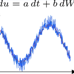
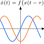
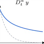
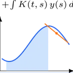
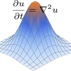
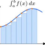
Initial-value problems, stochastic forcing, delay, fractional, integro, and PDE method-of-lines.

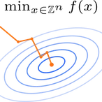
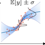
Continuous and constrained optimization, plus trajectory and adjoint methods.
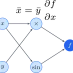
The lower-level primitives that the higher subsystems rest on, with first-class extension points.

The shared types, error model, and instrumentation that hold the rest of the workspace together.


● Composition
Fitting a parameterized ODE to noisy data with proper gradients usually means stitching together three or four libraries. In Numra it's a single workflow because every subsystem is built against the same types and the same error model.
use numra::ode::{Bdf, SolverOptions};
use numra::ode::sensitivity::{solve_forward_sensitivity, ParametricOdeSystem};
use numra::optim::{lm_minimize, LmOptions};

// Observed: a sample of the decaying state at t = 4.
let observed = 0.14;

// Parametric model: dy/dt = -k·y, with k unknown.
struct Decay { k: f64 }
impl ParametricOdeSystem<f64> for Decay {
    fn n_states(&self) -> usize  { 1 }
    fn n_params(&self) -> usize  { 1 }
    fn params(&self)   -> &[f64] { std::slice::from_ref(&self.k) }
    fn rhs_with_params(&self, _t: f64, y: &[f64], p: &[f64], dy: &mut [f64]) {
        dy[0] = -p[0] * y[0];
    }
}

// One Bdf solve of the augmented system gives state AND analytical sensitivity dy/dk.
let solve_with_sens = |k: &[f64]| {
    let sys = Decay { k: k[0] };
    solve_forward_sensitivity::<Bdf, f64, _>(
        &sys, 0.0, 4.0, &[1.0],
        &SolverOptions::default().rtol(1e-8).atol(1e-12),
    ).expect("augmented solve failed")
};

let residual = |k: &[f64], r: &mut [f64]| {
    let sol  = solve_with_sens(k);
    let last = sol.len() - 1;
    r[0] = sol.y_at(last)[0] - observed;
};
let jacobian = |k: &[f64], j: &mut [f64]| {
    let sol  = solve_with_sens(k);
    let last = sol.len() - 1;
    j[0] = sol.dyi_dpj(last, 0, 0);
};

let fit = lm_minimize(residual, jacobian, &[0.3], 1, &LmOptions::default())?;
println!("k = {:.4}  (final cost {:.2e})", fit.x[0], fit.f);
SolverOptions for ODE,
LmOptions for LM), but the
error types convert into NumraError
so the same ? operator
propagates across the whole pipeline.
Bdf with Radau5,
or the optimizer with a global search method, doesn't
require changing the integration code. Composition is at
the type level.
● Solver matrix
Every IVP solver in the workspace, with the properties that decide which one you reach for. Generated from the same metadata that drives the test suite — if a column says yes, there's a regression test enforcing it.
| Solver | Family | Order | Adaptive | Stiff | Dense out | Events | Notes |
|---|---|---|---|---|---|---|---|
| Explicit Runge–Kutta | |||||||
| DoPri5 | RK | 5(4) | ● | ○ | ● | ● | Dormand–Prince. Default for non-stiff. |
| Tsit5 | RK | 5(4) | ● | ○ | ● | ● | Tsitouras. Lower error coefficients than DoPri5. |
| Vern6 | RK | 6(5) | ● | ○ | ● | ● | High-order, smooth solutions. |
| Vern7 | RK | 7(6) | ● | ○ | ● | ● | Loose tolerances on long horizons. |
| Vern8 | RK | 8(7) | ● | ○ | ● | ● | Tight tolerances, smooth dynamics. |
| Vern9 | RK | 9(8) | ● | ○ | ● | ● | When you really need accuracy. |
| Implicit / stiff | |||||||
| Radau5 | IRK | 5 | ● | ● | ● | ● | A-stable, L-stable. The reference for stiff. |
| BDF | Multistep | 1–5 | ● | ● | ● | ● | Variable-order. Stiff and DAE-friendly. |
| ESDIRK4 | SDIRK | 4(3) | ● | ● | ● | ● | Diagonally-implicit, mildly stiff. |
| Stochastic | |||||||
| EulerMaruyama | SDE | 0.5 | ○ | ○ | ○ | ◐ | Strong order 0.5, weak 1.0. |
| Milstein | SDE | 1.0 | ○ | ○ | ○ | ◐ | Diagonal noise. |
| SRA / SRI | SDE | 1.5 | ● | ○ | ○ | ◐ | Adaptive, additive / Itô noise. |
● Benchmarks
Every benchmark figure ships with the commit, the CPU, the rustc version, and a one-line reproduction script. Plots that can't meet that bar don't ship — see the comparisons chapter for the full methodology.
solve_ivp(method='Radau')
● Architecture
Numra is organized in three layers. Each crate depends only on layers below it, so you can pull in just what you need without dragging in the whole numerical stack.
● Engineering posture
Three commitments across every release — provenance on every benchmark figure, regression tests against published invariants, and an explicit stability policy.
01 · Provenance
Every figure carries a SHA.
Every benchmark plot in the book is annotated with the Numra commit, CPU model, rustc version, and a link to the reproduction script. Plots without that bar don't ship.
Bench harness →02 · Tested
Invariants, not happy paths.
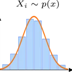
Convergence orders for ODE families, statistical bands for SDEs, golden-value LP/QP/MILP solutions, FFT round-trip, dense linear-solve smoke tests, and event localization.
Feature matrix →03 · Stability
Pre-1.0 churn is documented.
Until 1.0, breaking changes carry rationale in the changelog. After 1.0, deprecation cycles run across at least one minor version before removal.
Stability policy →● Where to start
Numra serves several distinct audiences. Choose the path that matches what brought you here.
"I want to install Numra and solve my first ODE."
Installation & first solve → Evaluator"I'm comparing Numra to SciPy and SciML for a project."
Read the book → Contributor"I want to understand the workspace architecture."
CONTRIBUTING & layer map → Researcher"I'm citing Numra in academic work."
BibTeX, DOI, CITATION.cff →@software{numra,
author = {Leblouba, Moussa},
title = {{Numra: Composable Numerical Methods for Rust}},
year = {2026},
publisher = {Spectral Automata},
version = {0.1.5},
doi = {10.5281/zenodo.20159709},
url = {https://doi.org/10.5281/zenodo.20159709},
}